

The same LLM session, even with identical model, parameters, prompts and responses, can incur substantially different costs depending on the inference provider that serves it. The gap comes from token pricing, provider prompt-caching behavior, and users’ request patterns. When those factors diverge, a cache-aware cost-arbitrage layer can reduce spend. The question is how large that reduction is and how reliable.
We benchmarked Auriko's cache-aware cost-arbitrage engine against five inference providers and an inference routing peer. The benchmark sent over 80,000 API requests to 37 models across three workload types. These requests form over 22,000 sessions. Auriko reduced dollar-weighted spend against six tested baselines: 32.8% against the routing peer (95% CI [30.6%, 34.9%]) and 7.7–38.3% across five single-provider baselines.
This report presents the benchmark results, explains the cost drivers behind the reduction, and documents the methodology, statistical tests, and robustness checks.
The Opportunity: Cost Dispersion Across Providers
Inference cost for the same requested model varies across providers. For some models we tested, the most expensive path costs 4× the cheapest for an identical request.
We compared 37 models across providers. For each model, we divided each provider's average cost by the lowest-cost provider's average cost and multiplied by 100. A score of 100 means cheapest. A score of 300 means three times the cost for the same request.
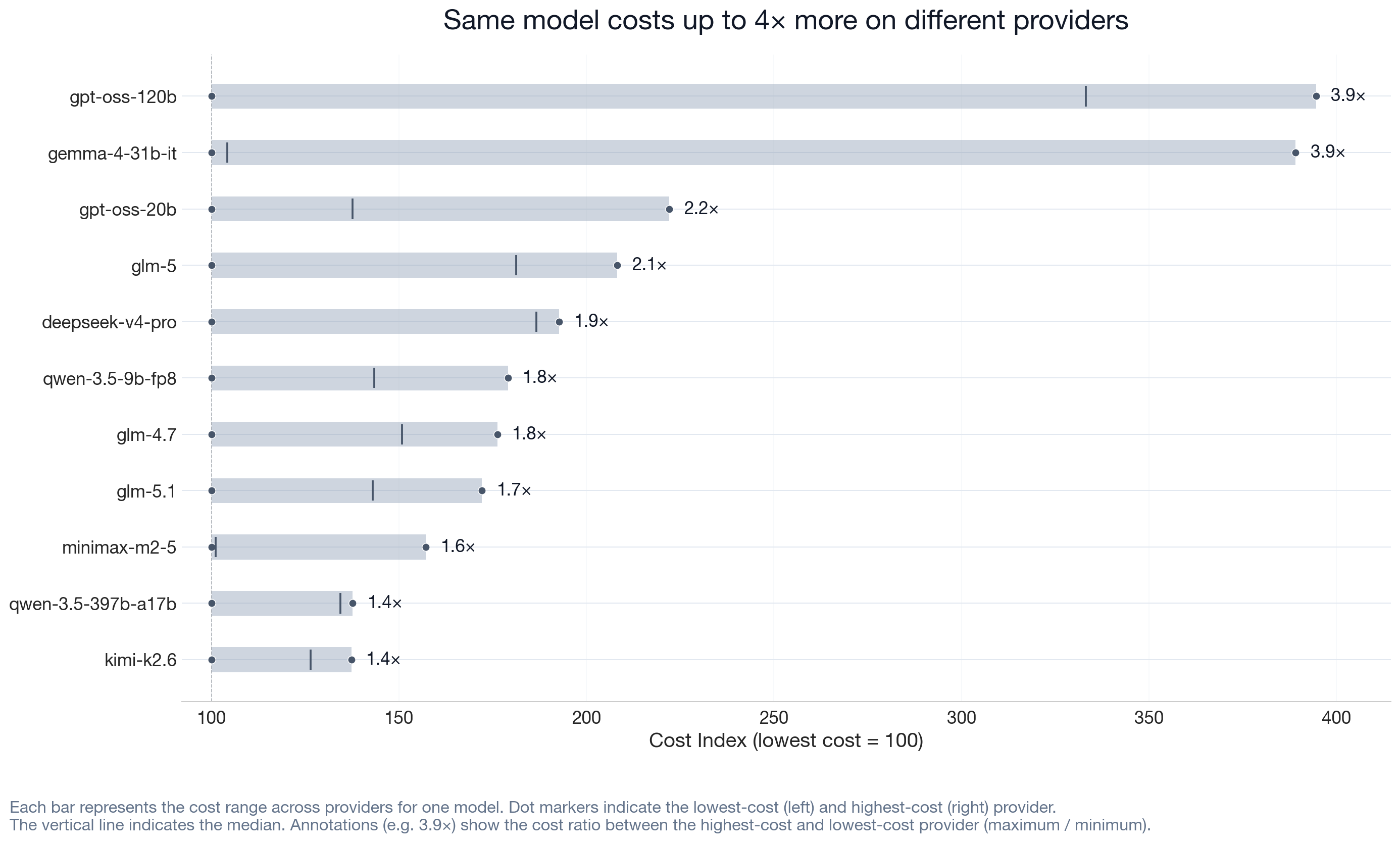
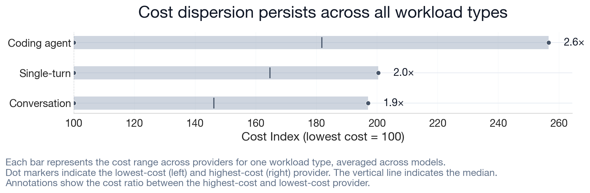
The variation appears across models in the study. The pattern holds across workload types. Coding agent workloads show the widest gap; single-turn and conversation workloads show comparable spreads (details in Robustness and Sensitivity).
This cost dispersion means that within the tested provider set, a cheapest provider choice exists for each measured workload. The rest of this report presents a statistical study of the cost reduction observed for Auriko's cache-aware routing approach. The next section describes how we conducted the study.
Experimental Design
This study adopts a matched-pairs design. For each model and workload combination, every call to Auriko and each comparator uses identical prompts. Request parameters — temperature, top-p, frequency penalty, presence penalty, and maximum output length — are held constant across all calls. Both sides are dispatched concurrently to control for time-of-day effects. Each combination is repeated multiple times. If either side of a pair errors, both sides are excluded before analysis.
Coverage
| Dimension | Coverage |
|---|---|
| Comparators | 1 routing peer + 5 inference providers |
| Models | 37 models |
| Workloads | Single-turn, multi-turn conversation, and multi-step coding agent sessions |
| Requests made | 80,634 API requests |
| LLM sessions | 22,416 sessions |
| Requested paired sessions | 10,752 |
| Clean paired target comparisons | 9,594 |
| Benchmark window | 2026-05-28 to 2026-06-07 UTC |
Requests made is the total number of individual API calls. LLM sessions group related calls into workload sessions, including multi-turn conversations and multi-step agent runs. Requested paired sessions are target-level session pairings before error exclusion; clean paired target comparisons are the same pairings after symmetric exclusion when either side errored.
Metric
Cost is the dollar amount returned by each API response. For session-level analysis, request costs are summed within each workload session. For the routing peer, cost is adjusted for their platform fee, matching what a user of that service effectively pays:
adjusted cost = API-returned cost × (1 + platform fee %)
Since Auriko charges no platform fees, no cost adjustment is needed.
Statistical Methods
| Method | Purpose |
|---|---|
| Stratified bootstrap (95% CI, 5,000 replicates, model + scenario strata) | Confidence intervals |
| Sign test (one-sided) | Directional evidence at the session level |
| Wilcoxon signed-rank test (one-sided) | Paired magnitude test |
| Holm–Bonferroni correction | Multiple-comparison control on model-level tests |
| Effect size (Hedges' g) | Standardized magnitude measure |
| Win rate inference (binomial + Wilson CI) | Session-level directional evidence |
Validity Controls
| Control | What it checks |
|---|---|
| Symmetric exclusion | Sessions with errors on either side are removed from both sides, preventing one-sided inflation |
| Output-volume normalization | Output costs scaled to match between sides |
| Output-volume filtering | Restricted to sessions where both sides produced similar output (±10%) |
| Error-inclusion test | Re-including error sessions to test whether exclusion materially changes the result |
The Evidence: Cost Reduction
The dispersion section showed that the same requested model can cost materially different amounts on different providers. This section presents Auriko's realized cost reduction against each comparator target.
Primary Findings
Auriko reduced dollar-weighted spend against six comparator targets, with target-level cost reduction ranging from 7.7% to 38.3%.
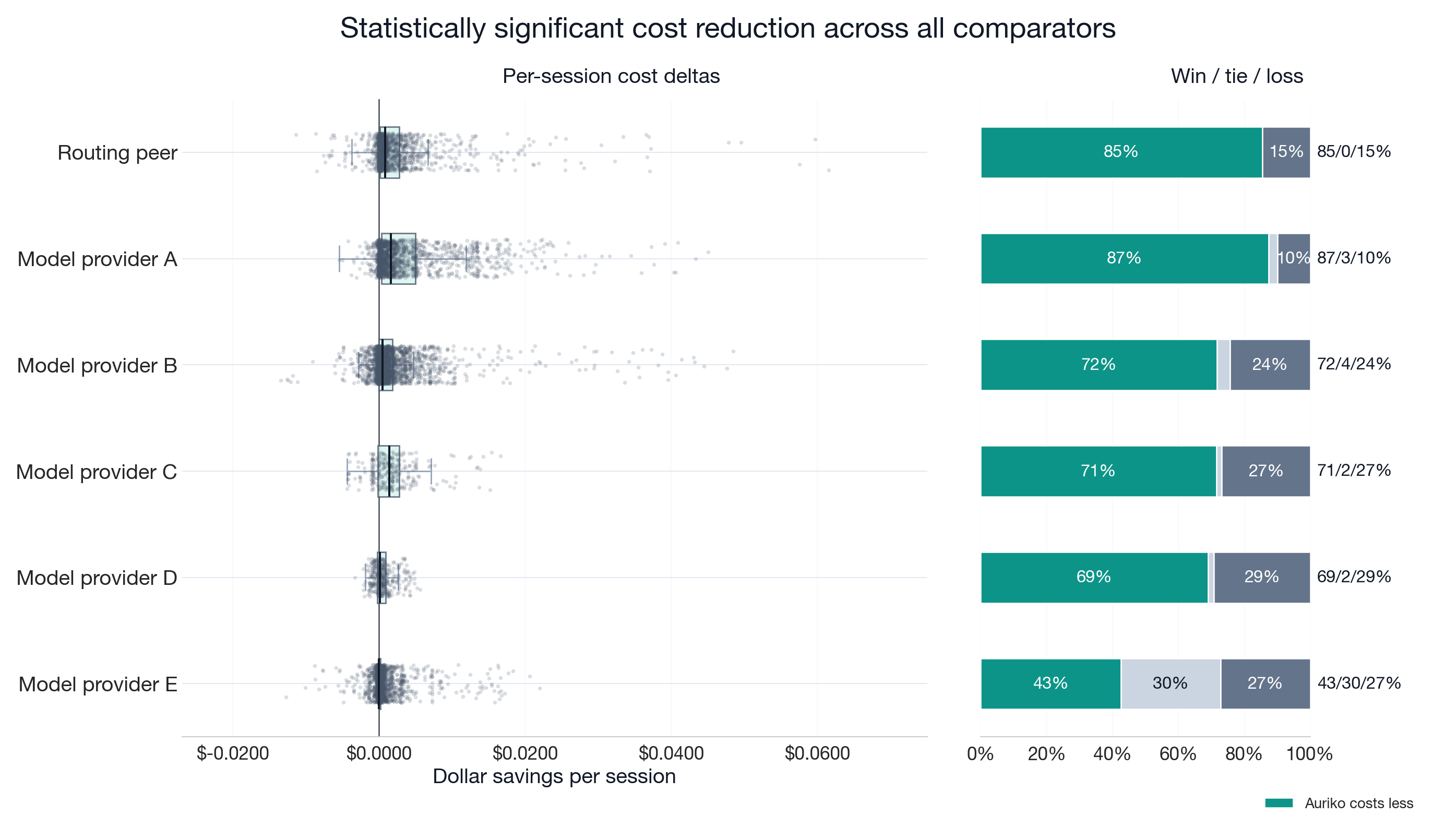
The chart below shows the distribution of session-level cost differences for each comparator target, together with the percentage of wins, ties, and losses — where a win is a session where Auriko costs less than the comparator. Auriko costs less in 61–90% of non-tie sessions across six targets.
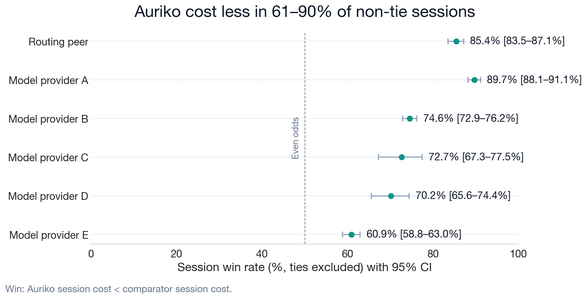
The chart below shows session win rates with 95% confidence intervals, ties excluded. Auriko costs less in the majority of non-tie sessions against each comparator target, with confidence intervals above the 50% even-odds line.
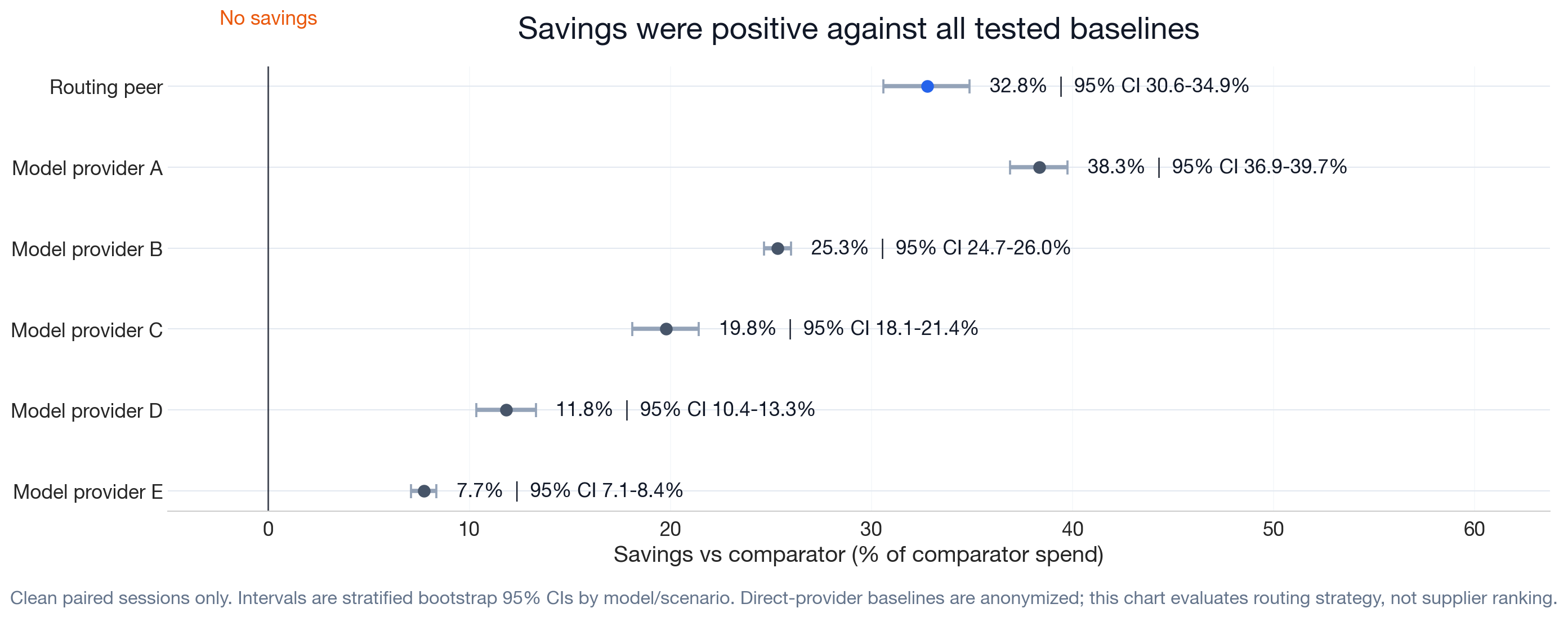
For each comparator target, the chart below shows dollar-weighted cost reduction with 95% confidence intervals. Cost reduction ranges from 7.7% (Model provider E) to 38.3% (Model provider A). Confidence intervals are computed via stratified bootstrap.
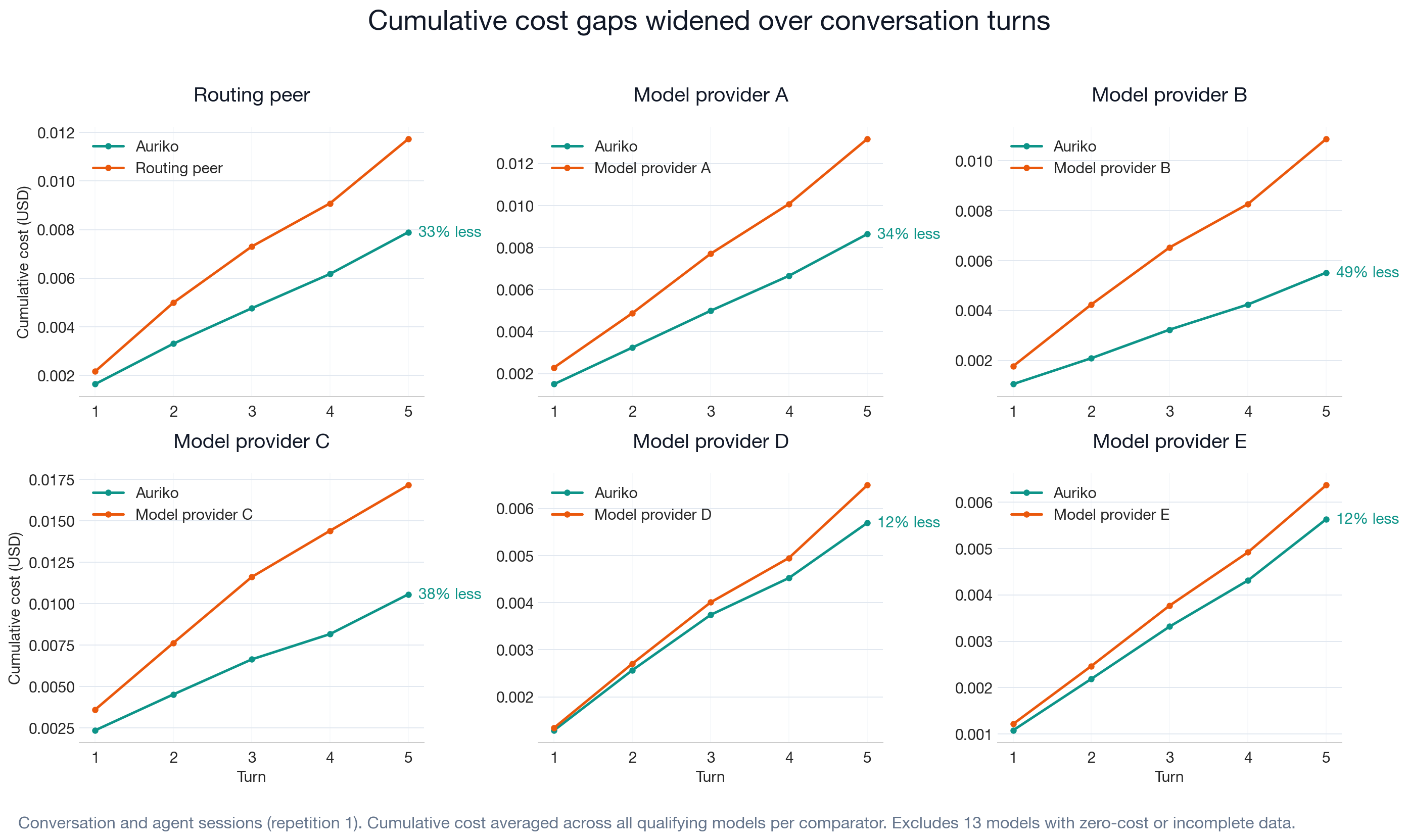
These panels show how cost accumulates over a multi-turn conversation. Each line is the average cumulative cost across models tested against that comparator. The gap between the lines is the cost reduction, and it widens with each turn, a pattern consistent with routing choices and reusable prompt context becoming more valuable over successive turns.
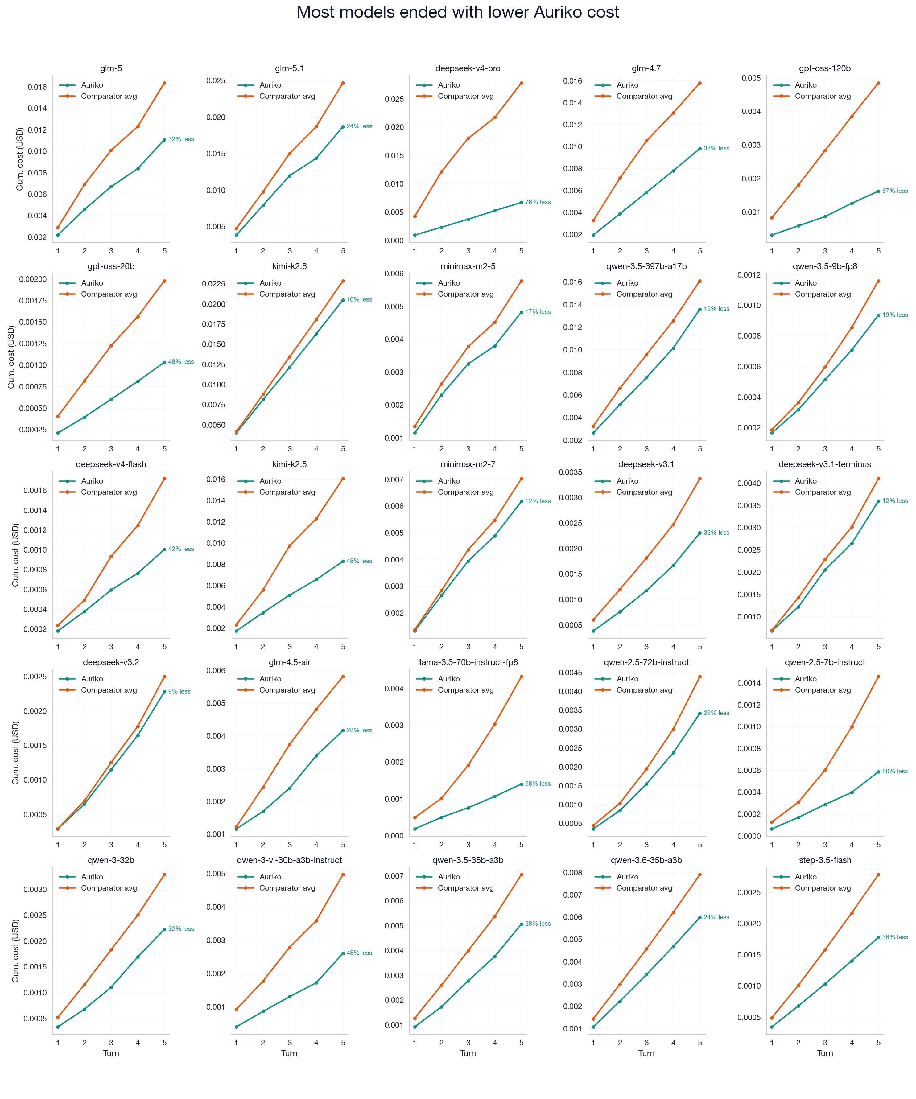
The per-model breakdown below shows the cumulative-cost gap is also visible at the individual-model level.
Cost Reduction Across Workloads
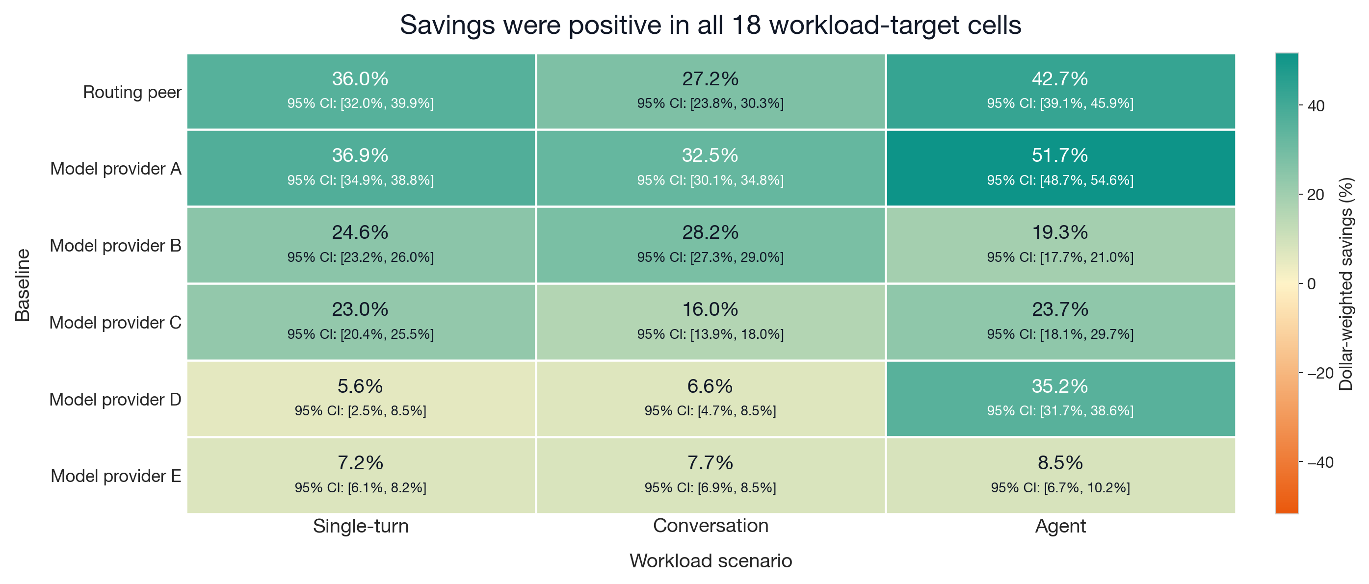
Each cell represents one comparator target paired with one workload scenario, annotated with the dollar-weighted cost reduction percentage for that pair. Color encodes magnitude. Cost reduction is positive across workload types and comparator targets.
For most targets, multi-turn workloads show larger cost reduction than single-turn requests, consistent with reusable prompt context becoming more valuable over successive turns.
Cost Reduction Across Models
A common objection to aggregate cost reduction is that one model with a large cost difference could drive the entire result. This subsection tests whether cost reduction is broad across the tested model set.
| Target | Models tested | Positive cost reduction | Holm-significant |
|---|---|---|---|
| Routing peer | 15 | 15 | 12 |
| Model provider A | 12 | 11 | 11 |
| Model provider B | 32 | 25 | 22 |
| Model provider C | 7 | 5 | 5 |
| Model provider D | 2 | 1 | 1 |
| Model provider E | 32 | 21 | 6 |
| Model provider cohort | 37 | 32 | 25 |
Holm-significant models survived Holm–Bonferroni multiple-comparison correction, a conservative family-wise correction across all model-level tests within the comparator group.
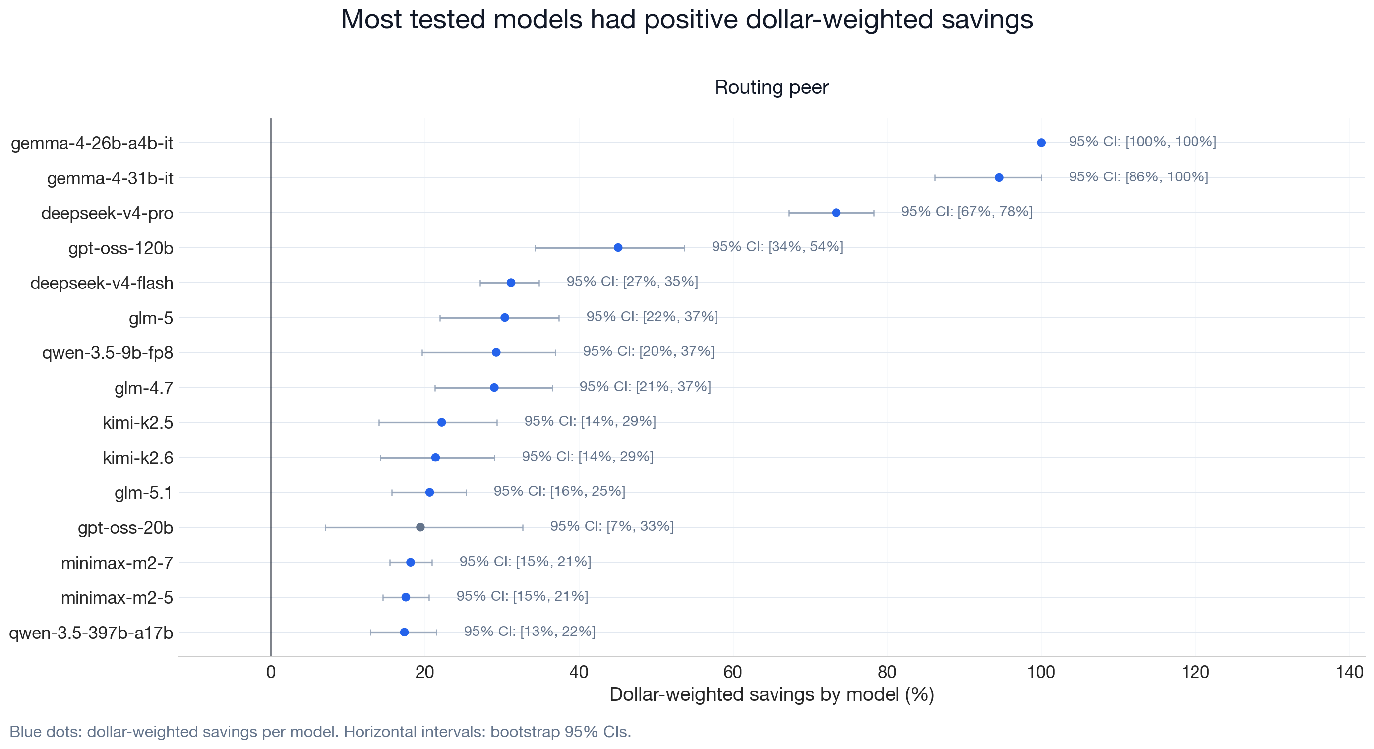
Each dot is one model's dollar-weighted cost reduction with a 95% bootstrap confidence interval. Blue markers indicate models that survived Holm–Bonferroni correction. Wider intervals reflect greater session-to-session cost variability for those models.
Statistical Tests
| Target | Sign test p | Wilcoxon p |
|---|---|---|
| Routing peer | < 0.001 | < 0.001 |
| Model provider A | < 0.001 | < 0.001 |
| Model provider B | < 0.001 | < 0.001 |
| Model provider C | < 0.001 | < 0.001 |
| Model provider D | < 0.001 | < 0.001 |
| Model provider E | < 0.001 | < 0.001 |
For each comparator target, we computed the session-level cost difference d = comparator cost − Auriko cost, where positive values indicate Auriko was cheaper. We tested the null hypothesis that Auriko has no lower session-level cost (H₀: the distribution of d is centered at zero) against the one-sided alternative (H₁: d is shifted positive) using two nonparametric tests.
The sign test counts non-tie sessions where Auriko costs less than the comparator versus more, and tests whether the lower-cost proportion exceeds 50%. The Wilcoxon signed-rank test incorporates magnitude by ranking the absolute differences, then testing whether positive ranks systematically outweigh negative ranks. Zero differences are discarded before ranking (Wilcox method). We report both tests because they are complementary: the sign test is robust to outliers (a single extreme session cannot drive the result), while the Wilcoxon is more powerful because it uses rank information.
Both tests reject H₀ at p < 0.001 for six comparator targets, with p-values ranging from 10⁻¹² to 10⁻²⁵⁴.
Summary Table
| Target | Dollar-weighted cost reduction | 95% CI | Win / Tie / Loss (%) |
|---|---|---|---|
| Routing peer | 32.8% | [30.6%, 34.9%] | 85.4 / 0.1 / 14.6 |
| Model provider A | 38.3% | [36.9%, 39.7%] | 87.4 / 2.6 / 10.0 |
| Model provider B | 25.3% | [24.7%, 26.0%] | 71.7 / 3.9 / 24.4 |
| Model provider C | 19.8% | [18.1%, 21.4%] | 71.4 / 1.7 / 26.9 |
| Model provider D | 11.8% | [10.4%, 13.3%] | 69.0 / 1.7 / 29.3 |
| Model provider E | 7.7% | [7.1%, 8.4%] | 42.5 / 30.2 / 27.3 |
Dollar-weighted cost reduction = (total comparator spend − total Auriko spend) / total comparator spend. 95% CI is a stratified bootstrap interval (5,000 replicates, model + scenario strata) around dollar-weighted cost reduction.
Model provider E has the narrowest target-level cost reduction and the highest tie rate. Its raw lower-cost rate is 42.5% because 30.2% of sessions are ties; excluding ties, Auriko costs less in 60.9% of non-tie sessions.
Dropping the highest-reduction direct baseline from the cohort, model provider cohort cost reduction remains at approximately 16.8%. The cohort result is not carried by a single anonymized baseline.
Cost Reduction Consistency
The preceding sections reported statistically significant cost differences across six comparators. Statistical significance provides evidence against the null hypothesis, but does not quantify magnitude — with sufficient sample size, even a negligible difference produces a significant p-value. Effect size measures how large the cost reduction is relative to session-to-session cost variability, independent of sample size.
We report Hedges' g: the mean per-session dollar difference (comparator minus Auriko) divided by its standard deviation, with a small-sample bias correction applied. Higher values indicate cost reduction that is consistent across sessions; lower values indicate cost reduction that is positive on average but more variable per session.
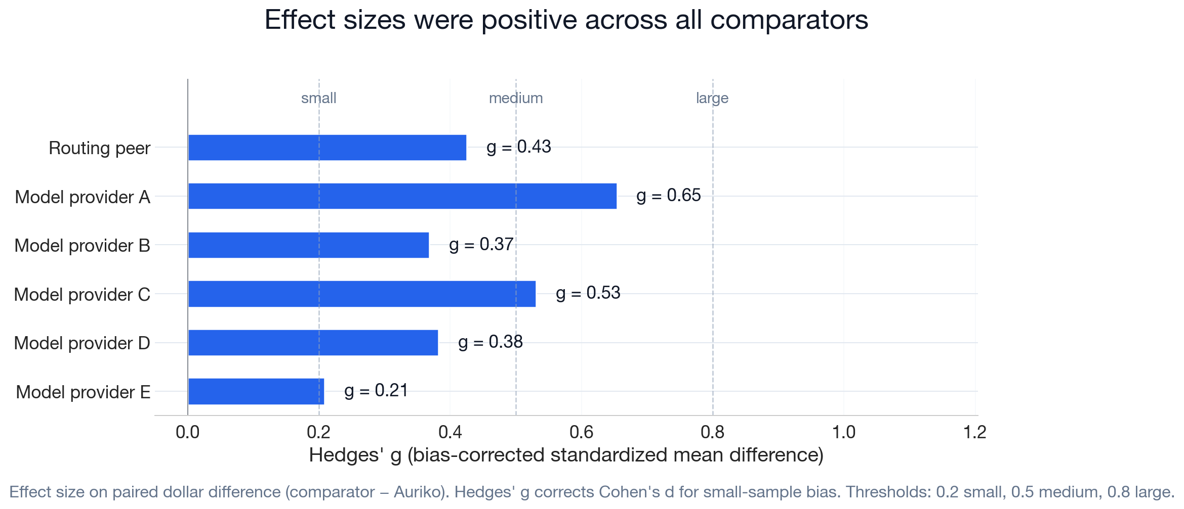
Hedges' g ranges from 0.21 (Model provider E, N = 3,077) to 0.65 (Model provider A, N = 1,647). Six comparators produce positive effect sizes.
The target-level results answer the magnitude question. The next question is which measured cost components are associated with this cost reduction.
The Mechanics: Cache-Aware Arbitrage
The actual cost of an LLM request depends on more than headline token price. On the provider side, five variables shape the realized cost: minimum token thresholds for cache activation, block granularity, cache expiration timing, write and storage costs, and context-length pricing tiers. On the user side, the workload pattern (prefix lengths, token reuse rates, request timing, and conversation depth) determines how effectively each provider's caching mechanics activate. The interaction between these two sides means the lowest-cost provider varies per request. For a full treatment of the cost model, see How Auriko Optimizes LLM Inference Cost.
This section examines two benchmark measurements that help explain Auriko's realized cost advantage: provider arbitrage and higher prompt-cache rate. First, we compare Auriko's routed cost with the tested provider cost range. Then, we look at prompt-cache hit rate improvements.
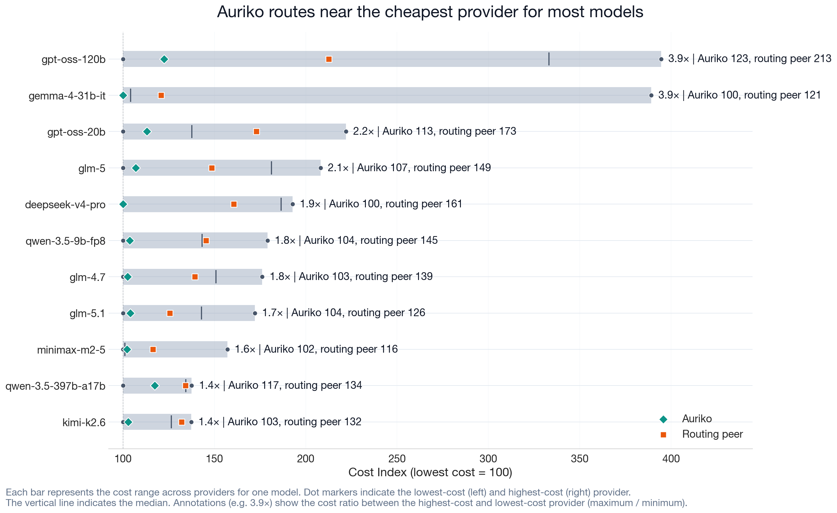
Provider Cost Arbitrage
The cost dispersion section showed that the same requested model can cost up to 4× more on different providers. This chart shows where Auriko's realized cost appears within that dispersion. For each model, the gray bar spans the cost range across the five tested single-provider baselines; the green diamond marks Auriko's realized cost, the orange square the routing peer's. Auriko's realized cost is near the low end of the range. The routing peer's cost is higher in the range.
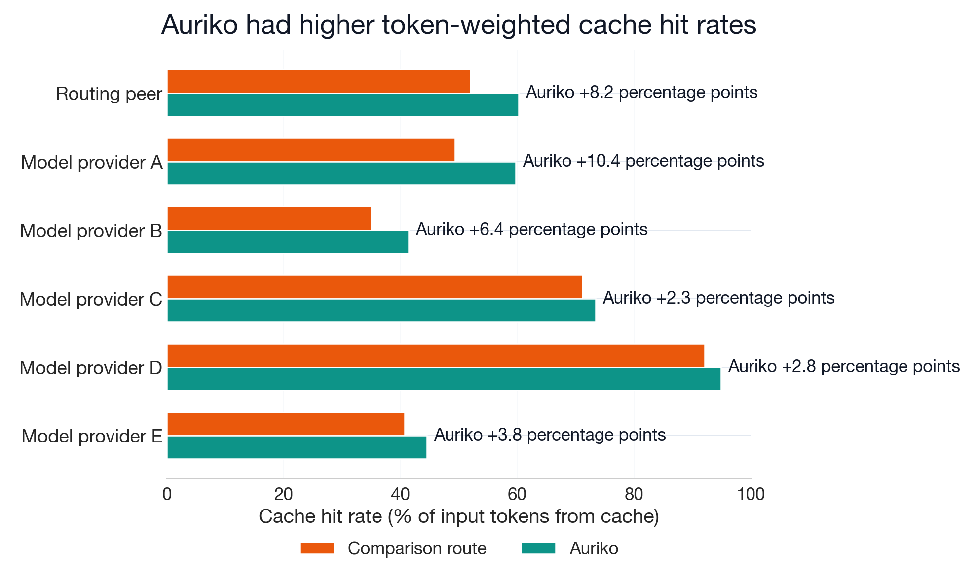
Prompt-Cache Hit Measures
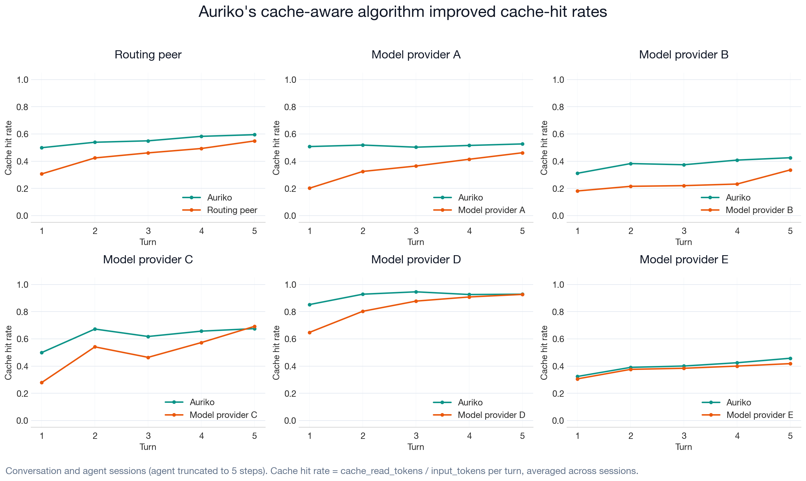
Providers charge a reduced rate for prompt tokens served from cache. Auriko had a higher token-weighted cache hit rate (cache-read tokens as a share of total input tokens) against six comparator targets, with deltas ranging from +2.3 to +10.4 percentage points.
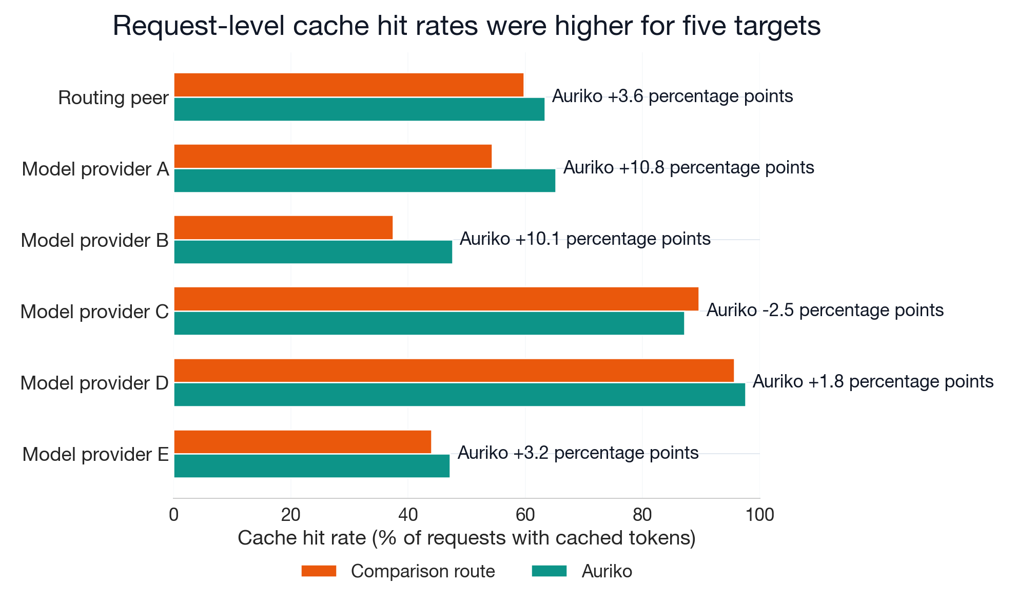
The previous chart measured the share of input tokens served from cache. This chart measures a different dimension: the share of requests with any cache hit. Auriko has a higher request-level hit rate against five of six targets. Model provider C is the exception, where the comparator leads by 2.5 percentage points.
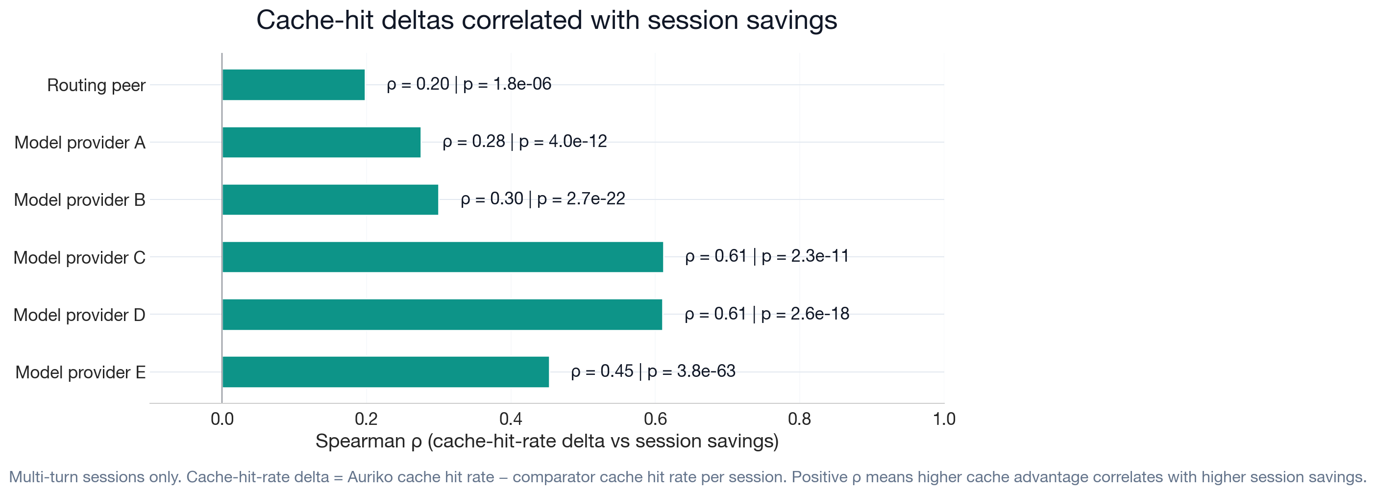
Session-level cache hit rate delta correlates positively with cost reduction across six comparator targets (Spearman ρ = 0.20 to 0.61).
Auriko's higher cache hit rate is consistent with selecting provider routes whose caching mechanics fit the measured usage pattern. Over successive conversation turns, the reusable prompt context grows and the measured cache-hit gap widens.
Robustness and Sensitivity
We tested the all-comparison aggregate result against 242 perturbations of the analysis sample: removing each scenario, comparator target, or model one at a time; re-including error sessions; normalizing completion-token costs; and restricting the analysis to sessions with similar output volumes. The result remained positive across every reported robustness-check family. The lowest aggregate estimate was 16.4% in the completion-matched subset.
Stress-Test Summary
The baseline dollar-weighted cost reduction across six comparator targets is 24.6% (95% CI [23.6%, 25.7%]). The table below reports the lowest estimate from each robustness-check family — the single variant in that family that produces the lowest cost reduction — along with its bootstrap confidence interval and the more conservative p-value from the sign test and Wilcoxon signed-rank test. It summarizes the all-comparison aggregate floor estimates, not all 242 robustness rows.
The full robustness package contains 242 rows across target-level, direct-provider-cohort, and all-comparison scopes: 24 scenario leave-one-out rows, 11 baseline leave-one-out rows, 175 model leave-one-out rows, 8 error-inclusion rows, and 24 completion-matched rows.
| Test | Controls for | Variants | Floor estimate | 95% CI | p-value |
|---|---|---|---|---|---|
| Leave-one-scenario-out | Workload-mix dependence | 3 | 23.6% (drop agent) | [22.8%, 24.4%] | < 10⁻¹⁸⁴ |
| Leave-one-baseline-out | Single-comparator dependence | 6 | 20.1% (drop Model provider A) | [19.3%, 20.9%] | < 10⁻³¹⁰ |
| Leave-one-model-out | Single-model dependence | 37 | 19.3% (drop deepseek-v4-pro) | [18.7%, 20.0%] | < 10⁻³⁰⁰ |
| Error-inclusion | Clean-success filter bias | 1 | 18.1% | [16.9%, 19.2%] | < 10⁻³⁰⁰ |
| Completion-matched (±10%) | Output-length variation | 1 (5,716 sessions) | 16.4% | [15.7%, 17.1%] | < 10⁻²⁹³ |
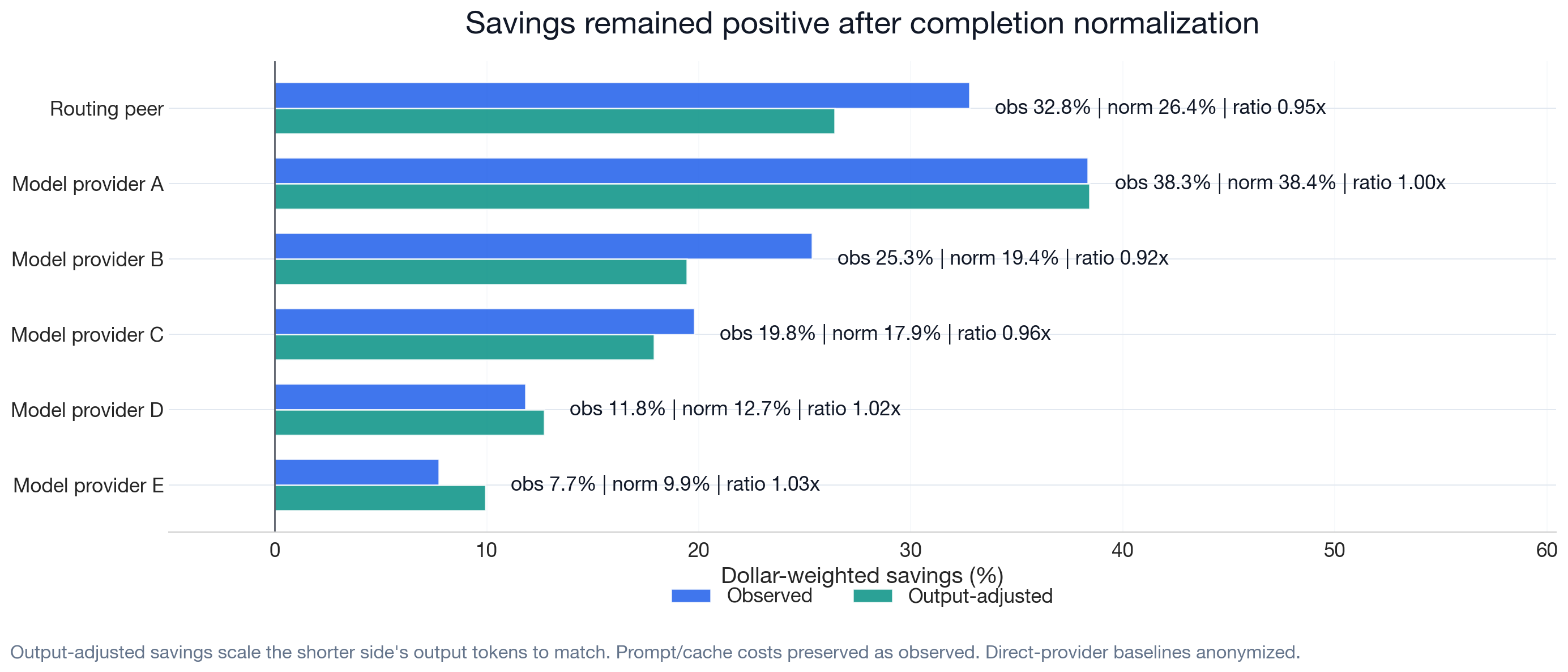
| Completion-normalized | Output-volume cost scaling | 1 | 22.6% | Per-target CIs above zero | All < 0.001 |
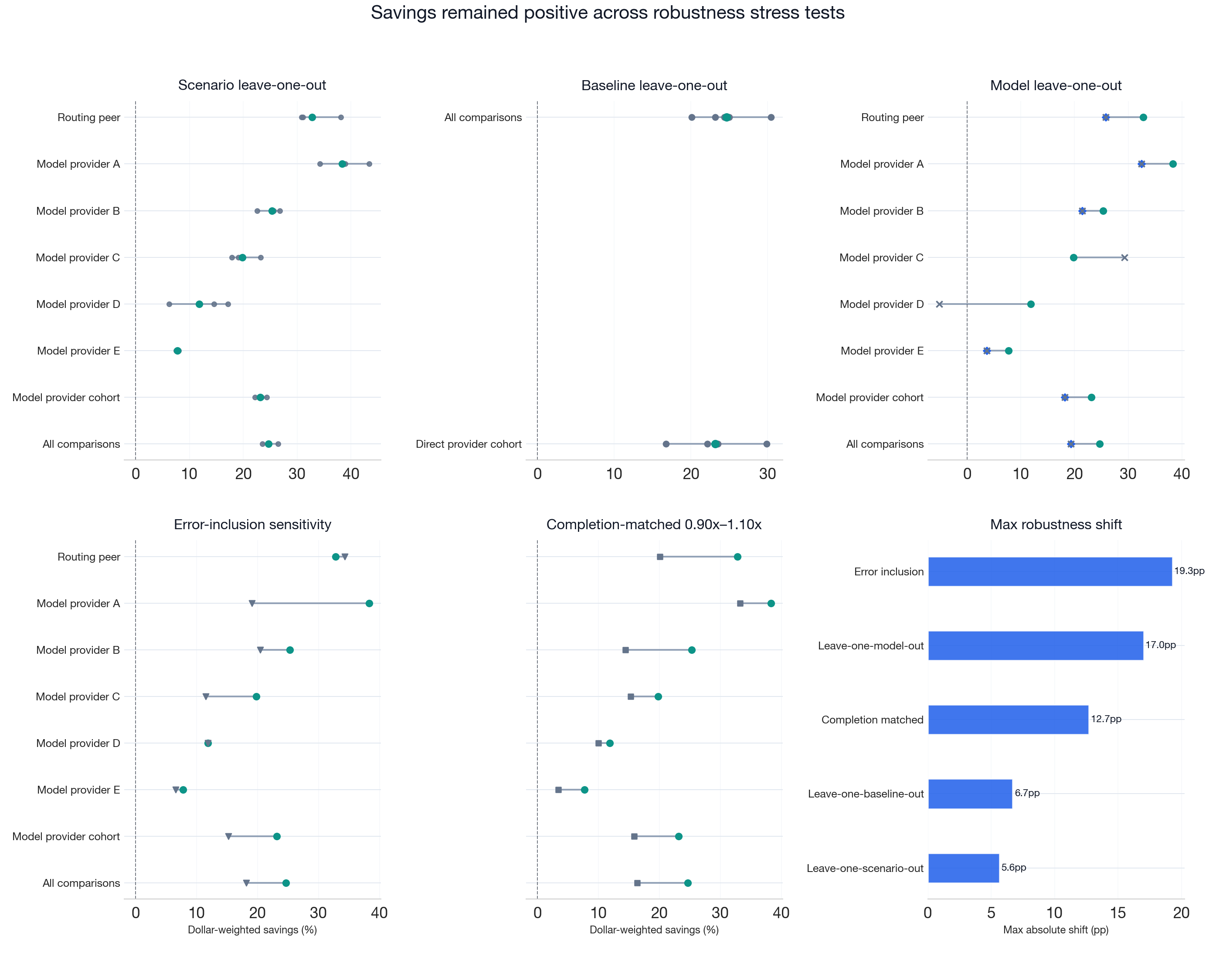
Five panels show per-target results under each stress test; the sixth shows the maximum shift from baseline for each test family. The table above reports the floor from each panel.
The error-inclusion row reintroduces 1,158 platform-complete sessions with at least one side marked as error; aggregate cost reduction remains 18.1%.
Leave-One-Out Stability
The three leave-one-out checks remove each scenario, comparator target, or model one at a time and recompute dollar-weighted cost reduction on the remaining sample. Scenario leave-one-out produces the tightest range (23.6%–26.4%), indicating that the result is not dependent on any one workload type in the leave-one-out check. Model leave-one-out shows the largest single-element influence: excluding deepseek-v4-pro yields 19.3% cost reduction (95% CI [18.7%, 20.0%]), reflecting that model's unusually large measured cost reduction in the benchmark.
Baseline leave-one-out ranges from 20.1% to 30.5%, depending on which comparator is excluded. This spread reflects the natural variation in per-target cost reduction, which ranges from 7.7% to 38.3%. Across scenario, baseline, and model leave-one-out checks, the aggregate CI lower bound remains above 18%.
Per-target detail for output-volume controls follows.
Completion Normalization
We test output-volume sensitivity by scaling output costs symmetrically: whichever side produced fewer completion tokens is scaled up to match the other side. Prompt and cache costs are preserved as observed. After normalization, cost reduction remains positive at 9.9–38.4% across targets, indicating that output-volume differences do not fully explain the result. Every per-target bootstrap interval remains above zero; the lowest lower bound is 9.5%. In the chart below, the ratio annotation is the output-token ratio: Auriko completion tokens divided by comparator completion tokens (see Glossary of Metrics).
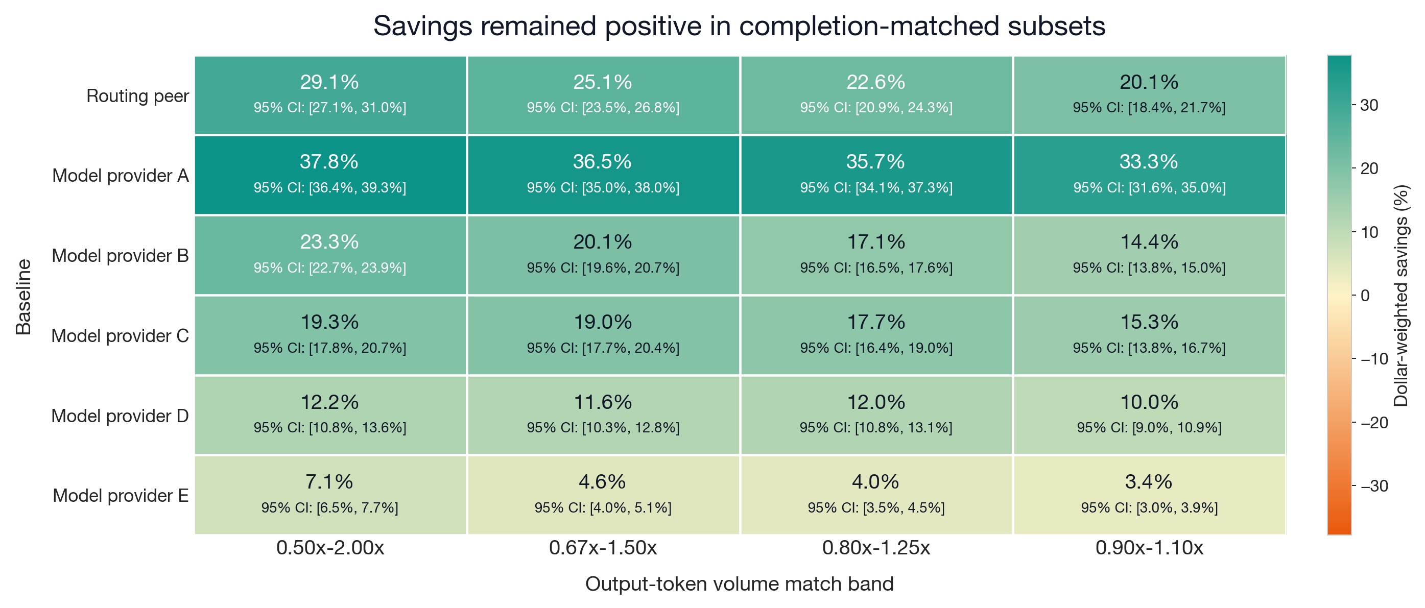
Completion-Matched Sensitivity
As a second output-volume check, we restrict the analysis to sessions where Auriko and the comparator produced similar output volumes. Even in the tightest band reported in the robustness table (±10%), cost reduction remains positive for most targets. A stricter ±5% output-matched diagnostic, tracked separately from the 242-row robustness table, retains 4,547 sessions (47.4% of paired sessions) and still produces 16.1% aggregate cost reduction. This is evidence that output-volume mismatch does not explain the full measured cost reduction.
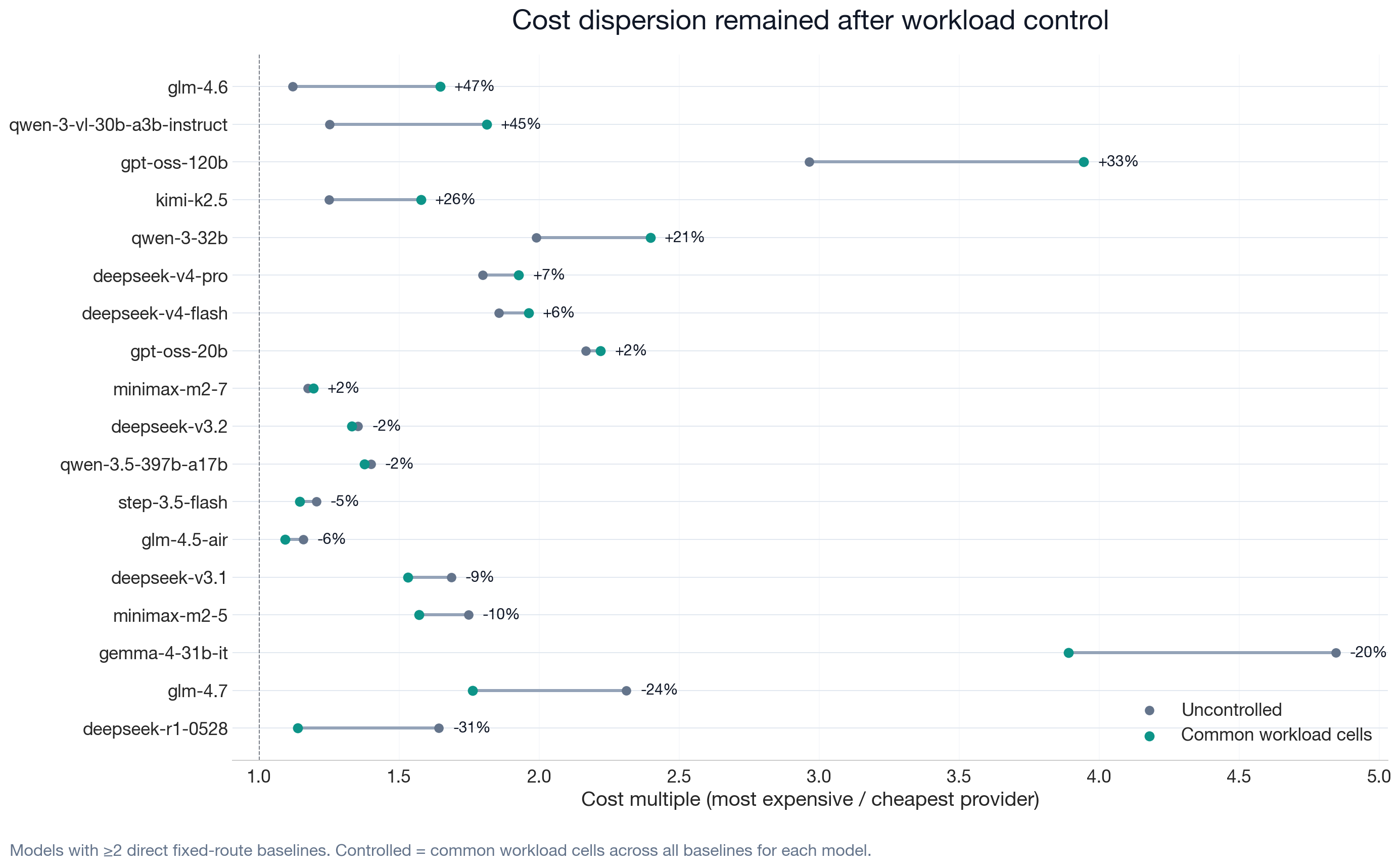
Workload-Controlled Dispersion
One objection to provider cost dispersion is that different providers might serve different workload mixes. We therefore compare uncontrolled provider spread against spread measured only within common workload cells: identical prompts sent to all providers for each model. The dispersion persists after this workload control, consistent with the cost-dispersion pattern shown earlier.
The controlled audit covers 36 models across 1,556 common workload cells. The median controlled spend multiple is 1.57×; 32 of 36 models remain above 1.1×, 20 remain above 1.5×, and 7 remain above 2×.
Across the reported all-comparison stress-test families, aggregate cost reduction ranged from 16.4% to 30.5%. Where aggregate confidence intervals are reported, their lower bounds remained above zero; completion-normalized per-target intervals also remained above zero. The next section defines the scope and boundaries of these results.
Scope of Results
This benchmark compared Auriko's realized costs against six comparator targets (one routing peer and five model providers) across 37 models and three workload types. The benchmark covers over 80,000 API requests forming over 22,000 sessions, collected over the benchmark window described in Experimental Design. Cost reduction was positive for each comparator target, each workload type, and 18 target-scenario cells, with dollar-weighted cost reduction ranging from 7.7% to 38.3% by target.
Comparator coverage. The benchmark tests six targets. The inference provider market includes providers not tested here.
Model coverage. 37 models are represented. Production workloads may include models outside this set. The model-level analysis shows cost reduction is distributed across models, not concentrated in a few.
Workload specificity. Cost reduction magnitudes are specific to this benchmark's workload mix. Different prompt lengths, conversation depths, or model distributions would produce different magnitudes.
Cost only. This benchmark measures cost. It does not measure latency, quality, or reliability differences across routes.
Validity analysis. Known limitations, confound controls, and threats to validity are examined in the Robustness and Sensitivity section.
Methodology
Metric definitions, experimental design, and statistical methods.
Glossary of Metrics
| Metric | Definition | Formula | Used in |
|---|---|---|---|
| Cache hit rate (request-level) | Share of requests with any cache-read tokens | requests with cache_read > 0 / successful requests | The Mechanics: Cache-Aware Arbitrage |
| Cache hit rate (token-weighted) | Cache hit rate weighted by total input tokens | Σ(cache_read_tokens) / Σ(input_tokens) | The Mechanics: Cache-Aware Arbitrage |
| Clean paired session | A session where both sides completed without error | Both sides non-null, non-error, symmetric exclusion | All sections |
| Completion-matched band | Subset where output-token ratios fall within a range | auriko_output / comp_output ∈ [lower, upper] | Robustness |
| Dollar-weighted cost reduction (%) | Aggregate cost reduction as share of comparator spend | (Σ comp_cost − Σ auriko_cost) / Σ comp_cost × 100 | The Evidence: Cost Reduction |
| Effect size (Hedges' g) | Bias-corrected standardized mean difference | mean(diffs) / sd(diffs), corrected for small N | The Evidence: Cost Reduction |
| Indexed spend (cheapest = 100) | Provider cost relative to cheapest for the same requested model | provider_cost / min(provider_costs) × 100 | Cost Dispersion Across Providers |
| Output-token ratio | Ratio of Auriko to comparator output tokens | auriko_completion_tokens / comp_completion_tokens | Robustness |
| Session win / tie / loss | Per-session outcome based on cost difference | Win: comp > auriko; Loss: auriko > comp; Tie: equal | The Evidence: Cost Reduction |
| Symmetric completion normalization | Scale shorter side's output tokens to match | Adjusts output cost component only; prompt/cache preserved | Robustness |
Statistical Methods
Confidence intervals. Percentile bootstrap on dollar-weighted cost reduction. 5,000 replicates, stratified by model and scenario. 2.5th–97.5th percentile (95% CI). Fixed seed for reproducibility.
Aggregate hypothesis tests. For each comparator target, session-level cost differences (d = comparator cost − Auriko cost) are tested with two one-sided nonparametric tests. The sign test counts non-tie sessions where Auriko costs less than the comparator versus more, and tests whether the lower-cost proportion exceeds 50%. The Wilcoxon signed-rank test ranks absolute differences and tests whether positive ranks systematically outweigh negative ranks.
Per-model hypothesis tests. Within each target, per-model cost differences are tested for normality (Shapiro-Wilk). Normal distributions use a paired t-test; non-normal distributions use a Wilcoxon signed-rank test. Both are two-sided.
Multiple comparisons. Holm–Bonferroni step-down procedure at α = 0.05 on per-model p-values within each target.
Effect size. Hedges' g: mean of paired cost differences divided by their standard deviation, with small-sample bias correction.
Win rate inference. Binomial test against H₀: win rate = 50% (ties excluded). Wilson score interval on session win rate.
Heterogeneity. Cochran's Q tests whether model-level cost reduction is homogeneous. I² estimates the proportion of variance due to true heterogeneity. τ² (DerSimonian-Laird) estimates between-model variance.
Limitations
| Limitation | Scope |
|---|---|
| Point-in-time snapshot | Results reflect the measurement window (2026-05-28 to 2026-06-07 UTC). Provider pricing and model availability change. |
| Workload representativeness | Production workloads may differ in prompt length, complexity, or domain. |
| Model selection | 37 models tested. Results apply to tested models only. |
| Geographic constraints | All sessions generated from a single geographic region. Provider-selection behavior may differ in other regions. |
| Routing algorithm evolution | Results reflect the algorithm version active during the measurement window. |